Getting Started

Install paste python package

You can install the package on pypi: https://pypi.org/project/paste-bio/

[1]:

import math
import time
import pandas as pd
import numpy as np
import scanpy as sc
import seaborn as sns
import matplotlib.pyplot as plt
import matplotlib.patches as mpatches
from matplotlib import style
import paste as pst

Read data and create AnnData object

[2]:

data_dir = './sample_data/'

# Assume that the coordinates of slices are named slice_name + "_coor.csv"
def load_slices(data_dir, slice_names=["slice1", "slice2", "slice3", "slice4"]):
    slices = []
    for slice_name in slice_names:
        slice_i = sc.read_csv(data_dir + slice_name + ".csv")
        slice_i_coor = np.genfromtxt(data_dir + slice_name + "_coor.csv", delimiter = ',')
        slice_i.obsm['spatial'] = slice_i_coor
        # Preprocess slices
        sc.pp.filter_genes(slice_i, min_counts = 15)
        sc.pp.filter_cells(slice_i, min_counts = 100)
        slices.append(slice_i)
    return slices

slices = load_slices(data_dir)
slice1, slice2, slice3, slice4 = slices

Each AnnData object consists of a gene expression matrx and spatial coordinate matrix.

[3]:

slice1.X

[3]:

array([[12.,  0.,  6., ...,  0.,  0.,  0.],
       [ 7.,  0.,  1., ...,  1.,  0.,  0.],
       [15.,  1.,  4., ...,  0.,  0.,  1.],
       ...,
       [ 0.,  0.,  0., ...,  0.,  0.,  0.],
       [ 1.,  0.,  0., ...,  0.,  0.,  0.],
       [ 5.,  0.,  1., ...,  1.,  0.,  0.]], dtype=float32)

[4]:

slice1.obsm['spatial'][0:5,:]

[4]:

array([[13.064,  6.086],
       [12.116,  7.015],
       [13.945,  6.999],
       [12.987,  7.011],
       [15.011,  7.984]])

Note, you can choose to label the spots however you want. In this case, we use the default coordinates.

[5]:

slice1.obs

[5]:

	n_counts
13.064x6.086	2181.0
12.116x7.015	2295.0
13.945x6.999	3375.0
12.987x7.011	2935.0
15.011x7.984	2964.0
...	...
21.953x24.847	541.0
20.98x24.963	860.0
20.063x24.964	508.0
19.007x25.045	626.0
21.957x25.871	2515.0

254 rows × 1 columns

[6]:

slice1.var

[6]:

	n_counts
GAPDH	2233.0
UBE2G2	78.0
MAPKAPK2	255.0
NDUFA7	96.0
ASNA1	172.0
...	...
DIP2C	31.0
LYPLA2	19.0
RGP1	24.0
BPGM	17.0
HPS6	16.0

7998 rows × 1 columns

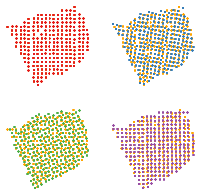
We can visualize the spatial coordinates of our slices using plot_slices.

[7]:

slice_colors = ['#e41a1c','#377eb8','#4daf4a','#984ea3']

fig, axs = plt.subplots(2, 2,figsize=(7,7))
pst.plot_slice(slice1,slice_colors[0],ax=axs[0,0])
pst.plot_slice(slice2,slice_colors[1],ax=axs[0,1])
pst.plot_slice(slice3,slice_colors[2],ax=axs[1,0])
pst.plot_slice(slice4,slice_colors[3],ax=axs[1,1])
plt.show()

../_images/notebooks_getting-started_13_0.png

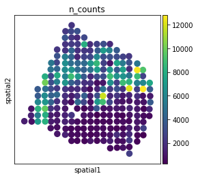
We can also plot using Scanpy’s spatial plotting function.

[8]:

sc.pl.spatial(slice1, color = "n_counts", spot_size = 1)

../_images/notebooks_getting-started_15_0.png

Pairwise Alignment

Run PASTE `pairwise_align`.

[9]:

start = time.time()

pi12 = pst.pairwise_align(slice1, slice2)
pi23 = pst.pairwise_align(slice2, slice3)
pi34 = pst.pairwise_align(slice3, slice4)

print('Runtime: ' + str(time.time() - start))

Using selected backend cpu. If you want to use gpu, set use_gpu = True.
Using selected backend cpu. If you want to use gpu, set use_gpu = True.
Using selected backend cpu. If you want to use gpu, set use_gpu = True.
Runtime: 0.5836582183837891

[10]:

pd.DataFrame(pi12)

[10]:

	0	1	2	3	4	5	6	7	8	9	...	240	241	242	243	244	245	246	247	248	249
0	0.003937	0.000000	0.000000	0.0	0.0	0.000000	0.000000	0.0	0.0	0.0	...	0.0	0.00000	0.000000	0.000000	0.0	0.000000	0.0	0.000000	0.000000	0.000000
1	0.000063	0.003874	0.000000	0.0	0.0	0.000000	0.000000	0.0	0.0	0.0	...	0.0	0.00000	0.000000	0.000000	0.0	0.000000	0.0	0.000000	0.000000	0.000000
2	0.000000	0.000000	0.000000	0.0	0.0	0.003937	0.000000	0.0	0.0	0.0	...	0.0	0.00000	0.000000	0.000000	0.0	0.000000	0.0	0.000000	0.000000	0.000000
3	0.000000	0.000126	0.003811	0.0	0.0	0.000000	0.000000	0.0	0.0	0.0	...	0.0	0.00000	0.000000	0.000000	0.0	0.000000	0.0	0.000000	0.000000	0.000000
4	0.000000	0.000000	0.000000	0.0	0.0	0.000000	0.003874	0.0	0.0	0.0	...	0.0	0.00000	0.000000	0.000000	0.0	0.000000	0.0	0.000000	0.000000	0.000000
...	...	...	...	...	...	...	...	...	...	...	...	...	...	...	...	...	...	...	...	...	...
249	0.000000	0.000000	0.000000	0.0	0.0	0.000000	0.000000	0.0	0.0	0.0	...	0.0	0.00000	0.000000	0.000000	0.0	0.000189	0.0	0.003622	0.000063	0.000063
250	0.000000	0.000000	0.000000	0.0	0.0	0.000000	0.000000	0.0	0.0	0.0	...	0.0	0.00000	0.000000	0.000000	0.0	0.000000	0.0	0.000000	0.003937	0.000000
251	0.000000	0.000000	0.000000	0.0	0.0	0.000000	0.000000	0.0	0.0	0.0	...	0.0	0.00000	0.001606	0.001953	0.0	0.000000	0.0	0.000378	0.000000	0.000000
252	0.000000	0.000000	0.000000	0.0	0.0	0.000000	0.000000	0.0	0.0	0.0	...	0.0	0.00189	0.000000	0.002047	0.0	0.000000	0.0	0.000000	0.000000	0.000000
253	0.000000	0.000000	0.000000	0.0	0.0	0.000000	0.000000	0.0	0.0	0.0	...	0.0	0.00000	0.000000	0.000000	0.0	0.000000	0.0	0.000000	0.000000	0.003937

254 rows × 250 columns

Sequential pairwise slice alignment plots

[11]:

pis = [pi12, pi23, pi34]
slices = [slice1, slice2, slice3, slice4]

new_slices = pst.stack_slices_pairwise(slices, pis)

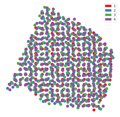
Now that we’ve aligned the spatial coordinates, we can plot them all on the same coordinate system.

[12]:

slice_colors = ['#e41a1c','#377eb8','#4daf4a','#984ea3']

plt.figure(figsize=(7,7))
for i in range(len(new_slices)):
    pst.plot_slice(new_slices[i],slice_colors[i],s=400)
plt.legend(handles=[mpatches.Patch(color=slice_colors[0], label='1'),mpatches.Patch(color=slice_colors[1], label='2'),mpatches.Patch(color=slice_colors[2], label='3'),mpatches.Patch(color=slice_colors[3], label='4')])
plt.gca().invert_yaxis()
plt.axis('off')
plt.show()

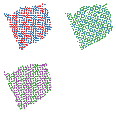
../_images/notebooks_getting-started_23_0.png

We can also plot pairwise layers together.

[13]:

slice_colors = ['#e41a1c','#377eb8','#4daf4a','#984ea3']

fig, axs = plt.subplots(2, 2,figsize=(7,7))
pst.plot_slice(new_slices[0], slice_colors[0], ax=axs[0,0])
pst.plot_slice(new_slices[1], slice_colors[1], ax=axs[0,0])
pst.plot_slice(new_slices[1], slice_colors[1], ax=axs[0,1])
pst.plot_slice(new_slices[2], slice_colors[2], ax=axs[0,1])
pst.plot_slice(new_slices[2], slice_colors[2], ax=axs[1,0])
pst.plot_slice(new_slices[3], slice_colors[3], ax=axs[1,0])
fig.delaxes(axs[1,1])
plt.show()

../_images/notebooks_getting-started_25_0.png

We can also plot the slices in 3-D.

[14]:

import plotly.express as px
import plotly.io as pio
pio.renderers.default='notebook'

slices_colors = ['#e41a1c','#377eb8','#4daf4a','#984ea3']

# scale the distance between layers
z_scale = 2

values = []
for i,L in enumerate(new_slices):
    for x,y in L.obsm['spatial']:
        values.append([x, y, i*z_scale, str(i)])
df = pd.DataFrame(values, columns=['x','y','z','slice'])
fig = px.scatter_3d(df, x='x', y='y', z='z',
              color='slice',color_discrete_sequence=slice_colors)
fig.update_layout(scene_aspectmode='data')
fig.show()

Center Alignment

First, we will read in and preprocess the data (if you ran pairwise_align above, it will be altered).

[15]:

slices = load_slices(data_dir)
slice1, slice2, slice3, slice4 = slices

Run PASTE `center_align`.

[16]:

slices = [slice1, slice2, slice3, slice4]
initial_slice = slice1.copy()
lmbda = len(slices)*[1/len(slices)]

Now, for center alignment, we can provide initial mappings between the center and original slices to PASTE to improve the algorithm. However, note this is optional.

[17]:

pst.filter_for_common_genes(slices)

b = []
for i in range(len(slices)):
    b.append(pst.match_spots_using_spatial_heuristic(slices[0].X, slices[i].X))

Filtered all slices for common genes. There are 6397 common genes.

[18]:

start = time.time()

center_slice, pis = pst.center_align(initial_slice, slices, lmbda, random_seed = 5, pis_init = b)

print('Runtime: ' + str(time.time() - start))

Using selected backend cpu. If you want to use gpu, set use_gpu = True.
Filtered all slices for common genes. There are 6397 common genes.

/home/max/Programs/envs/spatialOT/lib/python3.8/site-packages/sklearn/decomposition/_nmf.py:1076: ConvergenceWarning:

Maximum number of iterations 200 reached. Increase it to improve convergence.

Iteration: 0
Solving Pairwise Slice Alignment Problem.
Solving Center Mapping NMF Problem.

/home/max/Programs/envs/spatialOT/lib/python3.8/site-packages/sklearn/decomposition/_nmf.py:1076: ConvergenceWarning:

Maximum number of iterations 200 reached. Increase it to improve convergence.

Objective  1.42119034779904
Difference: 1.42119034779904

Iteration: 1
Solving Pairwise Slice Alignment Problem.
Solving Center Mapping NMF Problem.

/home/max/Programs/envs/spatialOT/lib/python3.8/site-packages/sklearn/decomposition/_nmf.py:1076: ConvergenceWarning:

Maximum number of iterations 200 reached. Increase it to improve convergence.

Objective  1.3973178012733354
Difference: 0.023872546525704585

Iteration: 2
Solving Pairwise Slice Alignment Problem.
Solving Center Mapping NMF Problem.
Objective  1.3967427058538635
Difference: 0.0005750954194718716

Runtime: 11.849297285079956

/home/max/Programs/envs/spatialOT/lib/python3.8/site-packages/sklearn/decomposition/_nmf.py:1076: ConvergenceWarning:

Maximum number of iterations 200 reached. Increase it to improve convergence.

Again, we can run center align without providing intial mappings below.

[19]:

# center_slice, pis = paste.center_align(initial_slice, slices, lmbda, random_seed = 5)

center_slice returns an AnnData object that also includes the low dimensional representation of our inferred center slice.

[20]:

center_slice.uns['paste_W']

[20]:

array([[2.23237598e-02, 1.14087162e+00, 9.58007337e-02, ...,
        7.89308199e-02, 1.35525808e-02, 1.29490388e-03],
       [4.23211589e-04, 3.82036845e-01, 1.95311398e-01, ...,
        3.97314769e-03, 1.30214566e-03, 6.30798032e-03],
       [1.59148391e-01, 1.59327668e-01, 7.87353959e-02, ...,
        2.27056510e-02, 6.34641837e-02, 1.40540096e-01],
       ...,
       [3.22691089e-02, 6.62650834e-04, 7.03813042e-02, ...,
        9.94040232e-04, 4.48582747e-03, 1.87143452e-01],
       [4.13513237e-02, 3.07151849e-03, 1.11811249e-01, ...,
        8.04589919e-03, 3.06158517e-04, 1.56736132e-01],
       [1.89361986e-01, 5.70979580e-05, 6.44658939e-03, ...,
        1.27158897e-04, 7.24546648e-03, 3.28253786e-02]])

[21]:

center_slice.uns['paste_H']

[21]:

array([[4.70866524e-01, 7.03703110e-02, 1.95729740e-02, ...,
        2.49784848e-02, 1.81434916e-02, 3.73244360e-02],
       [1.89843453e+00, 1.21216273e-01, 2.92930246e-01, ...,
        9.54992284e-02, 1.13389243e-01, 1.27972992e-02],
       [1.77937553e+00, 1.04479731e-01, 1.42932180e-01, ...,
        5.81047561e-02, 4.50576125e-02, 2.65283562e-02],
       ...,
       [2.71336626e+00, 1.83430076e-01, 5.47662565e-01, ...,
        5.24410308e-02, 5.50516787e-05, 6.20249102e-08],
       [9.65690784e-01, 1.49039550e-01, 9.42255518e-02, ...,
        8.73865104e-06, 5.63785405e-03, 5.51648331e-03],
       [5.50727274e+00, 2.28139877e-02, 2.63350947e-01, ...,
        5.88726839e-15, 7.02571694e-02, 0.00000000e+00]])

Center slice alignment plots

Next, we can use the outputs of center_align to align the slices.

[22]:

center, new_slices = pst.stack_slices_center(center_slice, slices, pis)

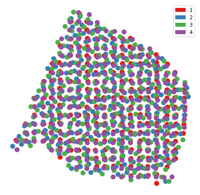
Now that we’ve aligned the spatial coordinates, we can plot them all on the same coordinate system. Note the center slice is not plotted.

[23]:

center_color = 'orange'
slices_colors = ['#e41a1c','#377eb8','#4daf4a','#984ea3']

plt.figure(figsize=(7,7))
pst.plot_slice(center,center_color,s=400)
for i in range(len(new_slices)):
    pst.plot_slice(new_slices[i],slices_colors[i],s=400)

plt.legend(handles=[mpatches.Patch(color=slices_colors[0], label='1'),mpatches.Patch(color=slices_colors[1], label='2'),mpatches.Patch(color=slices_colors[2], label='3'),mpatches.Patch(color=slices_colors[3], label='4')])
plt.gca().invert_yaxis()
plt.axis('off')
plt.show()

../_images/notebooks_getting-started_45_0.png

Next, we plot each slice compared to the center.

Note that since we used slice1 as the coordinates for the center slice, they remain the same, and thus we cannot see both in our plots below.

[24]:

center_color = 'orange'
slice_colors = ['#e41a1c','#377eb8','#4daf4a','#984ea3']

fig, axs = plt.subplots(2, 2,figsize=(7,7))
pst.plot_slice(center,center_color,ax=axs[0,0])
pst.plot_slice(new_slices[0],slice_colors[0],ax=axs[0,0])

pst.plot_slice(center,center_color,ax=axs[0,1])
pst.plot_slice(new_slices[1],slice_colors[1],ax=axs[0,1])

pst.plot_slice(center,center_color,ax=axs[1,0])
pst.plot_slice(new_slices[2],slice_colors[2],ax=axs[1,0])

pst.plot_slice(center,center_color,ax=axs[1,1])
pst.plot_slice(new_slices[3],slice_colors[3],ax=axs[1,1])
plt.show()

../_images/notebooks_getting-started_48_0.png

Gpu Implementation

POT allows us to write backend agnostic code, allowing us to use Numpy, Pytorch, etc to calculate our computations (https://pythonot.github.io/gen_modules/ot.backend.html).

We have updated our code to include gpu support for Pytorch.

First, you want to make sure you have torch installed. One way to check is by running:

[25]:

import ot
ot.backend.get_backend_list()

WARNING:absl:No GPU/TPU found, falling back to CPU. (Set TF_CPP_MIN_LOG_LEVEL=0 and rerun for more info.)

[25]:

[<ot.backend.NumpyBackend at 0x7fd6f387b160>,
 <ot.backend.TorchBackend at 0x7fd6f387b670>,
 <ot.backend.JaxBackend at 0x7fd8a44d2730>,
 <ot.backend.CupyBackend at 0x7fd6f3911b80>]

By default, you should have ot.backend.NumpyBackend(). To use our gpu, make sure you have ot.backend.TorchBackend().

If not, install torch: https://pytorch.org/

Note: From our tests, ot.backend.TorchBackend() is still faster than ot.backend.NumpyBackend() even if you ONLY use cpu, so we recommend trying it if you would like to speed up your calculations.

Now, assuming you have torch installed, we check to make sure you have access to gpu. PASTE automatically does this check for you, but it is still helpful to know if you want to debug why you can’t seem to access your gpu.

[26]:

import torch
torch.cuda.is_available()

[26]:

True

Running PASTE with gpu

Note: Since the breast dataset is small, cpu may actually be faster than gpu in this particular case. For larger datasets, you will see a greater improvement in gpu vs cpu.

First, we read in our data.

[27]:

data_dir = './sample_data/'

# Assume that the coordinates of slices are named slice_name + "_coor.csv"
def load_slices(data_dir, slice_names=["slice1", "slice2", "slice3", "slice4"]):
    slices = []
    for slice_name in slice_names:
        slice_i = sc.read_csv(data_dir + slice_name + ".csv")
        slice_i_coor = np.genfromtxt(data_dir + slice_name + "_coor.csv", delimiter = ',')
        slice_i.obsm['spatial'] = slice_i_coor
        # Preprocess slices
        sc.pp.filter_genes(slice_i, min_counts = 15)
        sc.pp.filter_cells(slice_i, min_counts = 100)
        slices.append(slice_i)
    return slices

slices = load_slices(data_dir)
slice1, slice2, slice3, slice4 = slices

Next, running with gpu is as easy as setting two parameters in our function.

[28]:

start = time.time()

pi12 = pst.pairwise_align(slice1, slice2, backend = ot.backend.TorchBackend(), use_gpu = True)
pi23 = pst.pairwise_align(slice2, slice3, backend = ot.backend.TorchBackend(), use_gpu = True)
pi34 = pst.pairwise_align(slice3, slice4, backend = ot.backend.TorchBackend(), use_gpu = True)

print('Runtime: ' + str(time.time() - start))

gpu is available, using gpu.
gpu is available, using gpu.
gpu is available, using gpu.
Runtime: 0.37587952613830566

[29]:

pd.DataFrame(pi12)

[29]:

	0	1	2	3	4	5	6	7	8	9	...	240	241	242	243	244	245	246	247	248	249
0	0.003937	0.000000	0.000000	0.0	0.0	0.000000	0.000000	0.0	0.0	0.0	...	0.0	0.00000	0.000000	0.000000	0.0	0.000000	0.0	0.000000	0.000000	0.000000
1	0.000063	0.003874	0.000000	0.0	0.0	0.000000	0.000000	0.0	0.0	0.0	...	0.0	0.00000	0.000000	0.000000	0.0	0.000000	0.0	0.000000	0.000000	0.000000
2	0.000000	0.000000	0.000000	0.0	0.0	0.003937	0.000000	0.0	0.0	0.0	...	0.0	0.00000	0.000000	0.000000	0.0	0.000000	0.0	0.000000	0.000000	0.000000
3	0.000000	0.000126	0.003811	0.0	0.0	0.000000	0.000000	0.0	0.0	0.0	...	0.0	0.00000	0.000000	0.000000	0.0	0.000000	0.0	0.000000	0.000000	0.000000
4	0.000000	0.000000	0.000000	0.0	0.0	0.000000	0.003874	0.0	0.0	0.0	...	0.0	0.00000	0.000000	0.000000	0.0	0.000000	0.0	0.000000	0.000000	0.000000
...	...	...	...	...	...	...	...	...	...	...	...	...	...	...	...	...	...	...	...	...	...
249	0.000000	0.000000	0.000000	0.0	0.0	0.000000	0.000000	0.0	0.0	0.0	...	0.0	0.00000	0.000000	0.000000	0.0	0.000189	0.0	0.003622	0.000063	0.000063
250	0.000000	0.000000	0.000000	0.0	0.0	0.000000	0.000000	0.0	0.0	0.0	...	0.0	0.00000	0.000000	0.000000	0.0	0.000000	0.0	0.000000	0.003937	0.000000
251	0.000000	0.000000	0.000000	0.0	0.0	0.000000	0.000000	0.0	0.0	0.0	...	0.0	0.00000	0.001606	0.001953	0.0	0.000000	0.0	0.000378	0.000000	0.000000
252	0.000000	0.000000	0.000000	0.0	0.0	0.000000	0.000000	0.0	0.0	0.0	...	0.0	0.00189	0.000000	0.002047	0.0	0.000000	0.0	0.000000	0.000000	0.000000
253	0.000000	0.000000	0.000000	0.0	0.0	0.000000	0.000000	0.0	0.0	0.0	...	0.0	0.00000	0.000000	0.000000	0.0	0.000000	0.0	0.000000	0.000000	0.003937